42 format data labels pane excel
Format a Map Chart - support.microsoft.com Select the data point of interest in the chart legend or on the chart itself, and in the Ribbon > Chart Tools > Format, change the Shape Fill, or change it from the Format Object Task Pane > Format Data Point > Fill dialog, and select from the Color Pallette: Other chart formatting Format Data Label: Label Position - Microsoft Community when you add labels with the + button next to the chart, you can set the label position. In a stacked column chart the options look like this: For a clustered column chart, there is an additional option for "Outside End" When you select the labels and open the formatting pane, the label position is in the series format section. Does that help?
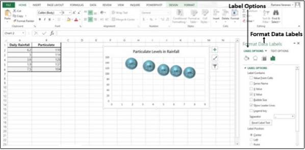
How to Add Data Labels to an Excel 2010 Chart - dummies On the Chart Tools Layout tab, click Data Labels→More Data Label Options. The Format Data Labels dialog box appears. You can use the options on the Label Options, Number, Fill, Border Color, Border Styles, Shadow, Glow and Soft Edges, 3-D Format, and Alignment tabs to customize the appearance and position of the data labels.
Format data labels pane excel
Advanced Excel - Leader Lines - tutorialspoint.com Step 3 − Move the data label. The Leader Line automatically adjusts and follows it. Format Leader Lines. Step 1 − Right-click on the Leader Line you want to format. Step 2 − Click on Format Leader Lines. The Format Leader Lines task pane appears. Now you can format the leader lines as you require. Step 3 − Click on the icon Fill & Line. Formatting data labels and printing pie charts on Excel for Mac 2019 ... Here's a work around I found for printing pie charts. Still can't find a solution for formatting the data labels. 1. When printing a pie chart from Excel for mac 2019, MS instructions are to select the chart only, on the worksheet > file > print. Excel is supposed to print the chart only (not the data ) and automatically fit it onto one page. Using Graphics to Represent Data Series (Microsoft Excel) Choose Format Data Series from the Context menu. Excel displays the Format Data Series task pane at the right side of the chart. In the task pane click the Fill & Line icon; it looks like a spilling paint bucket. Expand the Fill options by clicking the small triangle next to the Fill heading. (See Figure 2.) Figure 2. The Fill options of the ...
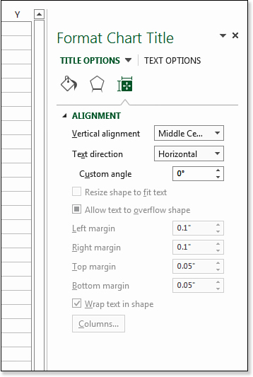
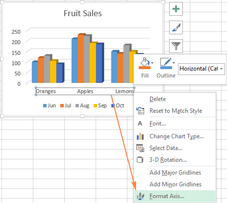
Format data labels pane excel. How to Customize Your Excel Pivot Chart Data Labels - dummies Excel displays the Format Data Labels pane. Check the box that corresponds to the bit of pivot table or Excel table information that you want to use as the label. For example, if you want to label data markers with a pivot table chart using data series names, select the Series Name check box. File format reference for Word, Excel, and PowerPoint - Deploy … 30.09.2021 · The binary file format for Excel 2019, Excel 2016, Excel 2013, and Excel 2010 and Office Excel 2007. This is a fast load-and-save file format for users who need the fastest way possible to load a data file. Supports VBA projects, Excel 4.0 macro sheets, and all the new features that are used in Excel. But, this is not an XML file format and is therefore not optimal … How to Add Data Labels to Scatter Plot in Excel (2 Easy Ways) - ExcelDemy By our previous action, a task pane named Format Data Labels opens. Firstly, click on the Label Options icon. In the Label Options, check the box of Value From Cells. Then, select the cells in the B5:B14 range in the Select Data Label Range box. These cells contain the Name of the individuals which we Format elements of a chart - support.microsoft.com Right-click the chart axis, and click Format Axis. In the Format Axis task pane, make the changes you want. You can move or resize the task pane to make working with it easier. Click the chevron in the upper right. Select Move and then drag the pane to a new location. Select Size and drag the edge of the pane to resize it.
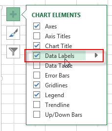
File format reference for Word, Excel, and PowerPoint ... Sep 30, 2021 · The Excel 5.0/95 Binary file format. .xlsb : Excel Binary Workbook : The binary file format for Excel 2019, Excel 2016, Excel 2013, and Excel 2010 and Office Excel 2007. This is a fast load-and-save file format for users who need the fastest way possible to load a data file. Supports VBA projects, Excel 4.0 macro sheets, and all the new ... Excel 2019 & 365 Tutorial Formatting Data Labels Microsoft Training FREE Course! Click: Learn about Formatting Data Labels in Microsoft Excel at . A clip from Mastering Excel ... Add or remove data labels in a chart - support.microsoft.com Right-click the data series or data label to display more data for, and then click Format Data Labels. Click Label Options and under Label Contains, select the Values From Cells checkbox. When the Data Label Range dialog box appears, go back to the spreadsheet and select the range for which you want the cell values to display as data labels. Dynamically Label Excel Chart Series Lines - My Online Training … 26.09.2017 · Select the Format tab (In Excel 2007 & 2010 it’s the Layout tab) Click on the drop down; Select the first label series: Step 4: Add the Labels. Excel 2013/2016 Click the + icon beside the chart as shown below (Note: for Excel 2007/2010 go to Layout tab) Data Labels; More Options; This will open the Format Data Labels pane/dialog box where you can choose …
Pie Chart in Excel - Inserting, Formatting, Filters, Data Labels Click on the Instagram slice of the pie chart to select the instagram. Go to format tab. (optional step) In the Current Selection group, choose data series "hours". This will select all the slices of pie chart. Click on Format Selection Button. As a result, the Format Data Point pane opens. How to change chart axis labels' font color and size in Excel? Note: You can also enter the code of #,##0_ ;[Red]-#,##0 into the Format Code box and click the Add button too. By the way, you can change the color name in the format code, such as #,##0_ ;[Blue]-#,##0. 3. Close the Format Axis pane or Format Axis dialog box. Now all negative labels in the selected axis are changed to red (or other color ... Prepare your Excel data source for a Word mail merge Format numerical data in Excel Format any numerical data like percentages or currency values in any new or existing data source in Excel that you intend to use in a Word mail merge. To preserve numeric data you've formatted as a percentage or as currency during a mail merge, follow the instructions in the "Step 2: Use Dynamic Data Exchange (DDE) for a mail merge" … How to hide zero data labels in chart in Excel? - ExtendOffice In the Format Data Labelsdialog, Click Numberin left pane, then selectCustom from the Categorylist box, and type #""into the Format Codetext box, and click Addbutton to add it to Typelist box. See screenshot: 3. Click Closebutton to close the dialog. Then you can see all zero data labels are hidden.
Using the Excel 2013 Interface | Using the Ribbon | InformIT
How to add data labels from different column in an Excel chart? Right click the data series, and select Format Data Labels from the context menu. 3. In the Format Data Labels pane, under Label Options tab, check the Value From Cells option, select the specified column in the popping out dialog, and click the OK button. Now the cell values are added before original data labels in bulk. 4.

Format Data Label Options for Charts in PowerPoint 2013 for Windows
Format Chart Axis in Excel – Axis Options 14.12.2021 · Formatting a Chart Axis in Excel includes many options like Maximum / Minimum Bounds, Major / Minor units, Display units, Tick Marks, Labels, Numerical Format of the axis values, Axis value/text direction, and more. However, there are a lot more formatting options for the chart axis, in this blog, we will be working with the axis options and Size, and properties.
Excel charts: add title, customize chart axis, legend and data labels
How to format axis labels as thousands/millions in Excel? - ExtendOffice Right click at the axis you want to format its labels as thousands/millions, select Format Axisin the context menu. 2. In the Format Axisdialog/pane, click Number tab, then in theCategorylist box, select Custom, and type[>999999] #,,"M";#,"K"into Format Codetext box, and click Addbutton to add it toTypelist. See screenshot: 3.

How to hide zero data labels in chart in Excel?
Edit titles or data labels in a chart - support.microsoft.com The first click selects the data labels for the whole data series, and the second click selects the individual data label. Right-click the data label, and then click Format Data Label or Format Data Labels. Click Label Options if it's not selected, and then select the Reset Label Text check box. Top of Page

Module1
How to add data labels from different column in an Excel chart? In the Format Data Labels pane, under Label Options tab, check the Value From Cells option, select the specified column in the popping out dialog, and click the OK button. Now the cell values are added before original data labels in bulk. 4. Go ahead to untick the Y Value option (under the Label Options tab) in the Format Data Labels pane.

Excel 3-D Pie Charts
Excel 2016 Tutorial Formatting Data Labels Microsoft Training Lesson FREE Course! Click: about Formatting Data Labels in Microsoft Excel at . A clip from Mastering Excel M...
Change the format of data labels in a chart - Office Support
Add a DATA LABEL to ONE POINT on a chart in Excel You can now configure the label as required — select the content of the label (e.g. series name, category name, value, leader line), the position (right, left, above, below) in the Format Data Label pane/dialog box. To format the font, color and size of the label, now right-click on the label and select 'Font'. Note: in step 5. above, if ...

Create Budget vs Actual Variance chart in Excel
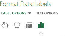
Change the format of data labels in a chart To get there, after adding your data labels, select the data label to format, and then click Chart Elements > Data Labels > More Options. To go to the appropriate area, click one of the four icons ( Fill & Line , Effects , Size & Properties ( Layout & Properties in Outlook or Word), or Label Options ) shown here.
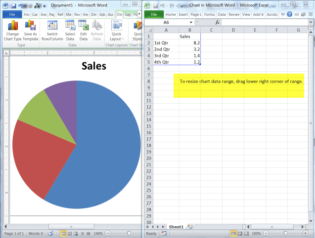
How to Add a Pie Chart in a Word 2010 Document | Daves Computer Tips
Format Chart Axis in Excel – Axis Options - Excel Unlocked Analyzing Format Axis Pane. Right-click on the Vertical Axis of this chart and select the "Format Axis" option from the shortcut menu. This will open up the format axis pane at the right of your excel interface. Thereafter, Axis options and Text options are the two sub panes of the format axis pane.

Advanced Excel Richer Data Labels in Advanced Excel Functions Tutorial 03 December 2020 - Learn ...
How to Create Mailing Labels in Excel | Excelchat B. If we do this, when next we open the document, MS Word will ask where we want to merge from Excel data file. We will click Yes to merge labels from Excel to Word. Figure 26 - Print labels from excel (If we click No, Word will break the connection between document and Excel data file.) C. Alternatively, we can save merged labels as usual text.

Format Data Label Options for Charts in PowerPoint 2013 for Windows
How to add data labels from different column in an Excel chart? In the Format Data Labels pane, under Label Options tab, check the Value From Cells option, select the specified column in the popping out dialog, and click the OK button. Now the cell values are added before original data labels in bulk. 4. Go ahead to untick the Y Value option (under the Label Options tab) in the Format Data Labels pane.

Directly Labeling Excel Charts | PolicyViz
Excel Charts - Quick Formatting - tutorialspoint.com The Format pane by default appears on the right-side of the chart. Step 1 − Click on the chart. Step 2 − Right-click the horizontal axis. A drop-down list appears. Step 3 − Click Format Axis. The Format pane for formatting axis appears. The format pane contains the task pane options. Step 4 − Click the Task Pane Options icon.

How to Customize Your Excel Pivot Chart Data Labels - dummies
Formatting Data Labels Ribbon: On the Series tab, in the Properties group, open the Data Labels drop-down menu and select More Data Labels Options to open the Format Labels dialog box ...

Excel charts: add title, customize chart axis, legend and data labels
Advanced Excel - Leader Lines - tutorialspoint.com Step 3 − Move the data label. The Leader Line automatically adjusts and follows it. Format Leader Lines. Step 1 − Right-click on the Leader Line you want to format. Step 2 − Click on Format Leader Lines. The Format Leader Lines task pane appears. Now you can format the leader lines as you require. Step 3 − Click on the icon Fill & Line.
Add or remove data labels in a chart - Office Support
How to Print Labels from Excel - Lifewire 05.04.2022 · How to Print Labels From Excel . You can print mailing labels from Excel in a matter of minutes using the mail merge feature in Word. With neat columns and rows, sorting abilities, and data entry features, Excel might be the perfect application for entering and storing information like contact lists.Once you have created a detailed list, you can use it with other …
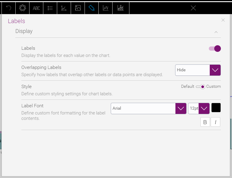
Format chart labels | Community
How to Print Labels from Excel - Lifewire Select Mailings > Write & Insert Fields > Update Labels . Once you have the Excel spreadsheet and the Word document set up, you can merge the information and print your labels. Click Finish & Merge in the Finish group on the Mailings tab. Click Edit Individual Documents to preview how your printed labels will appear. Select All > OK .
Advanced Excel - Краткое руководство - CoderLessons.com
Format Data Labels in Excel- Instructions - TeachUcomp, Inc. To do this, click the "Format" tab within the "Chart Tools" contextual tab in the Ribbon. Then select the data labels to format from the "Chart Elements" drop-down in the "Current Selection" button group. Then click the "Format Selection" button that appears below the drop-down menu in the same area.
Excel Charts - Free Excel Tutorial
Change the format of data labels in a chart Data labels make a chart easier to understand because they show details about a data series or its individual data points. For example, in the pie chart below, without the data labels it would be difficult to tell that coffee was 38% of total sales. You can format the labels to show specific labels elements like, the percentages, series name, or category name.
Post a Comment for "42 format data labels pane excel"