39 row labels in excel pivot table
› pivot-table-tips-and-tricks101 Advanced Pivot Table Tips And Tricks You Need To Know Apr 25, 2022 · With all options unchecked the pivot table is empty of row headers, banded rows, column headers and banded columns. Adding Row Headers. Adding Banded Rows. Adding Column Headers. Adding Banded Columns. Refresh Your Data excel - Custom row labels in PivotTable - Stack Overflow 1 you can give nicknames to the fields that you are checking which populate the pivot table. If you go the pivot table data and right click you can change the value field settings to give a custom name to a row/series but I do not know about individual data points. path: pivot table data => right click => select Field Settings => edit custom name.
Pivot Table - How to fill down data in row labels? - MrExcel Message Board Hi Excel gurus, In a pivot table, when we have more than one field under 'Row Labels', we get blank rows inserted in between. Is there a way, we can fill these blanks with the previous rows' entries? I know this can be done with Go To Special > Blanks feature, but this doesn't work on a pivot. Any idea how this can be done? Thanks much!

Row labels in excel pivot table
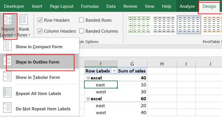
Remove row labels from pivot table • AuditExcel.co.za Click on the Pivot table Click on the Design tab Click on the report layout button Choose either the Outline Format or the Tabular format If you like the Compact Form but want to remove 'row labels' from the Pivot Table you can also achieve it by Clicking on the Pivot Table Clicking on the Analyse tab Pivot Table "Row Labels" Header Frustration - Microsoft Tech Community Public Sector. Internet of Things (IoT) Azure Partner Community. Expand your Azure partner-to-partner network. Microsoft Tech Talks. Bringing IT Pros together through In-Person & Virtual events. MVP Award Program. Find out more about the Microsoft MVP Award Program. How to Customize Your Excel Pivot Chart Data Labels - dummies The Data Labels command on the Design tab's Add Chart Element menu in Excel allows you to label data markers with values from your pivot table. When you click the command button, Excel displays a menu with commands corresponding to locations for the data labels: None, Center, Left, Right, Above, and Below. None signifies that no data labels ...
Row labels in excel pivot table. get a row label from pivot table - Microsoft Tech Community Creating PivotTable add data to data model by checking Create PivotTable and after that convert it to cube formulas. Now you may take these formulas and convert it to form you need, for example in H3 it could be =CUBEVALUE( "ThisWorkbookDataModel", CUBEMEMBER("ThisWorkbookDataModel", " [Measures]. › excelpivottableselectHow to Select Parts of Excel Pivot Table Jul 12, 2021 · Select any cell in the pivot table; On the Excel Ribbon, under Pivot Table Tools, click the Options tab; In the Actions group, click the Move PivotTable command ; In the Move dialog box, select New Worksheet, or select a location on an existing sheet. Click OK; Select Labels in Pivot Table Move Row Labels in Pivot Table - Excel Pivot Tables Move Row Labels in Pivot Table When you add fields to the row labels area in a pivot table, the field's items are automatically sorted. See how you can manually move those labels, to put them in a different order. There's a video and written steps below. In the screen shot below, the districts are listed alphabetically, from Central to West. › 2009/10/20 › pivot-table-errorPivot Table Error: Excel Field Names Not Valid Oct 20, 2009 · To help identify the problem pivot table, use the “List All Pivot Table – Headings” macro from my Contextures website. Copy the code from that page, and paste it into a regular code module, then run the macro. The macro lists each pivot table in the file, with the following information: Worksheet name; Pivot Table name; Pivot Cache index ...
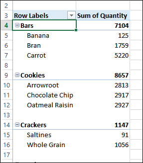
Pivot Table Row Labels In the Same Line - Beat Excel! After creating a pivot table in Excel, you will see the row labels are listed in only one column. But, if you need to put the row labels on the same line to view the data more intuitively and clearly as following screenshots shown. How could you set the pivot table layout to your need in Excel? My pivot table is showing "" on label : excel I am about to inherit a spreadsheet from another department in a month time but I was horrified when I opened the spreadsheet. The spreadsheet is riddled with obsolete links, REF! errors, unnecessarily tables/charts, badly named ranges/arrays in the hundreds (etc list1, list2...You get the idea) which made tracing formulas a near impossible task, hidden rows/columns which I have no idea why ... Use column labels from an Excel table as the rows in a Pivot Table First, we can try unpivoting your data: Highlight your current table, including the headers. Then from the Data section of the ribbon, select From Table. Highlight all the columns containing data, but not the Year column, and then select Unpivot Columns. Close the dialog and keep the changes. Excel should place the unpivoted data into a new ... How to make row labels on same line in pivot table? Please do as follows: 1. Click any cell in your pivot table, and the PivotTable Tools tab will be displayed. 2. Under the PivotTable Tools tab, click Design > Report Layout > Show in Tabular Form, see screenshot: 3. And now, the row labels in the pivot table have been placed side by side at once, see screenshot:
How do I show row labels in different columns in PivotTable? Select a cell in the pivot table. On the Ribbon, click the Design tab, and click Report Layout….To show the item labels in every row, for a specific pivot field: Right-click an item in the pivot field. In the Field Settings dialog box, click the Layout & Print tab. Add a check mark to Repeat item labels, then click OK. › documents › excelHow to filter date range in an Excel Pivot Table? - ExtendOffice Now you have filtered out the specified date range in the pivot table. (2) If you want to filter out a dynamic date range in the pivot table, please click the arrow beside Row Labels, and then in the drop-down list click Date Filters > This Week, This month, Next Quarter, etc. as you need. Pivot Table Row Labels - Microsoft Community If you go to PivotTable Tools > Analyze > Layout > Report Layout > Show in Tabular Form, your column headers will be used for the row labels. Every once in a while there's a sudden gust of gravity... Report abuse Was this reply helpful? Yes No A. User Replied on December 19, 2017 In reply to SmittyPro1's post on December 19, 2017 Automatic Row And Column Pivot Table Labels - How To Excel At Excel The first thing to do is put your cursor somewhere in your data list Select the Insert Tab Hit Pivot Table icon Next select Pivot Table option Select a table or range option Select to put your Table on a New Worksheet or on the current one, for this tutorial select the first option Click Ok
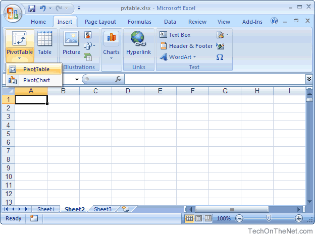
MS Excel 2007: How to Create a Pivot Table
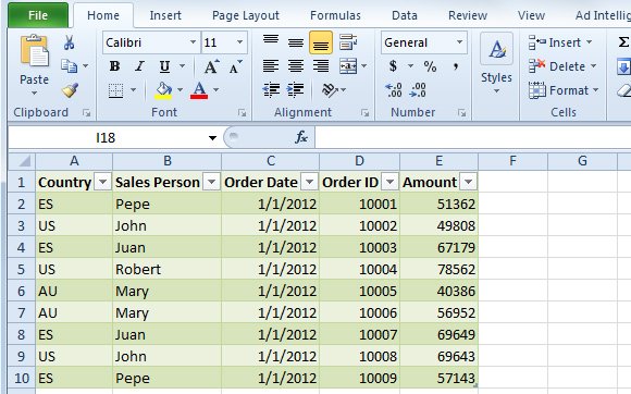
Pivot table row labels side by side - Excel Tutorials You can copy the following table and paste it into your worksheet as Match Destination Formatting. Now, let's create a pivot table ( Insert >> Tables >> Pivot Table) and check all the values in Pivot Table Fields. Fields should look like this. Right-click inside a pivot table and choose PivotTable Options…. Check data as shown on the image below.
How to Repeat Row Labels in Pivot Table - Free Excel Tutorial
How to Use Excel Pivot Table Label Filters In an Excel pivot table, you might want to hide one or more of the items in a Row field or Column field. To do that, you could click the drop down arrow for the Row or Column Labels, to see the list of pivot items in that pivot field. Then, in the list, remove the check mark for items you want to remove.
How to use Excel Pivot Tables
Excel Pivot Table Row labels - Stack Overflow 1 Answer. Sorted by: 0. Right click on the pivot, go to PivotTable Options, Display Tab. Click on "Classic Pivot Table Layout". Go to each field (column), right click, field settings, layout & print tab. Click on "Repeat Item Labels". That should give you the table you're looking for.

How to group by week in pivot table?
How to Create Pivot Tables in Microsoft Excel Open any data you want in Excel. I'm using Students marks as an example. Click the Insert tab and select Pivot Table. The Create PivotTable dialogue box comes up. Select the range of data and select New Worksheet if you want to display the pivot table in a new worksheet. I recommend displaying the Pivot Table in a new worksheet. Click OK.
Better Format for Pivot Table Headings – Excel Pivot Tables
How to rename group or row labels in Excel PivotTable? To rename Row Labels, you need to go to the Active Field textbox. 1. Click at the PivotTable, then click Analyze tab and go to the Active Field textbox. 2. Now in the Active Field textbox, the active field name is displayed, you can change it in the textbox.
Excel VBA: Pivot Table Tricks to Make You a Star
How to Add Rows to a Pivot Table: 9 Steps (with Pictures) Click Add under "Rows." It's in the left side of the pivot table editor. A list of fields will expand on the menu. 4 Click the name of the field you want to add as a row. Rows are usually non-numeric fields, such as category names and/or column headers. Once you select a field, a new row or rows will be added for the items in that field.
How to ungroup dates in an Excel pivot table?
How to Create Pivot Tables in Excel You can also create a Pivot Table in Excel using an outside data source, such as Access. ... Add a row field. When creating a Pivot Table, you are essentially sorting your data by rows and columns. ... For example, setting your Store field as the filter instead of a Row Label will allow you to select each store to see individual sales totals ...

23 things you should know about Excel pivot tables | Exceljet
Pivot table row labels in separate columns • AuditExcel.co.za So when you click in the Pivot Table and click on the DESIGN tab one of the options is the Report Layout. Click on this and change it to Tabular form. Your pivot table report will now look like the bottom picture and will be easier to use in other areas of the spreadsheet and in our opinion is also easier to read. Who wants to be a ...
Post a Comment for "39 row labels in excel pivot table"